
Work with Cognite Data Fusion
Level 1 explained what CDF is. Level 2 makes you productive: you will bring data in, shape it, model it, link it, query it with Python, put it in front of users, and secure it. Every module ends with something you have actually built.
- Level 1 complete (or the official CDF Fundamentals certificate). You should be able to draw Figure 3.1 (the six stations) and Figure 4.2 (the Core Data Model) from memory.
- Basic Python (variables, loops, functions,
pip install) and basic SQL (SELECT … JOIN … WHERE). If you are rusty, 2 hours on any beginner tutorial is enough. - Somewhere to work: your company CDF project (ideally a dev project with write access) and the free sandbox from Level 1 · 5.5. Exercises say which one they need.
The Level 2 roadmap
We follow the data. Modules 1–2 get data in and shape it; 3–4 model and link it; 5 programs against it; 6–8 deliver it to people and secure it. The running example stays the same as Level 1: boiler feed pump BFP-1A in Unit 2.
Getting data in: extractors & extraction pipelines
⏱ 3 h- The four kinds of extractor and when to use each
- How the PI, OPC UA and DB extractors are configured
- What RAW looks like from the inside and when to bypass it
- How to register, monitor and get alerted on an extraction pipeline
1.1 Four kinds of extractor
| Kind | Runs where | Typical sources | You maintain |
|---|---|---|---|
| Cognite self-hosted | Your server/VM/container next to the source (Windows service, Linux, Docker) | PI (AVEVA), OPC UA, OPC Classic, databases (ODBC), file shares, SAP, Documentum… | The VM, the YAML config, upgrades |
| Cognite hosted | Inside CDF — nothing on premises | MQTT brokers, Kafka, Azure Event Hub, REST APIs (polling) | Only the configuration in the UI |
| Custom (extractor-utils) | Wherever you run Python/.NET | Anything with an API or a file: lab systems, vendor portals, Modbus gateways | The code (Level 3) |
| Connectors | Cloud-to-cloud | Microsoft Fabric / OneLake, Databricks, simulators | Two-way sync settings |
A self-hosted extractor is a courier you employ at the plant: it walks into the historian room, copies what changed, and drives it to the cloud on a schedule. A hosted extractor is a mailbox at the cloud's door: anything that can already reach the internet (an MQTT broker, an IoT hub) just drops data in. Couriers are needed when the source sits behind a plant firewall — which is most OT systems.
1.2 The big three for OT: PI, OPC UA, DB
All Cognite extractors share one design: a YAML config file with a cognite section (where to send, how to authenticate), a source section (where to read), and an extractor section (behaviour: state store, buffering, batch sizes). Here is an illustrative DB-extractor config that lands an equipment table in RAW — the exact keys are in each extractor's docs, but the shape is always this:
# db-extractor config (illustrative — check the extractor docs for exact keys)
version: 3
logger:
  console: { level: INFO }

cognite:
  project: hnm-dev
  host: https://westeurope-1.cognitedata.com
  idp-authentication:                       # service principal, never a personal login
    token-url: https://login.microsoftonline.com/${TENANT_ID}/oauth2/v2.0/token
    client-id: ${CLIENT_ID}
    secret: ${CLIENT_SECRET}
    scopes: [ https://westeurope-1.cognitedata.com/.default ]
  extraction-pipeline: { external-id: ep_cmms_equipment }   # ties runs to a pipeline (1.4)

extractor:
  state-store: { local: { path: state.json } }             # remembers "where was I" between runs

databases:
  - name: cmms
    connection-string: "Driver={ODBC Driver 18 for SQL Server};Server=cmms-db;Database=maint;Trusted_Connection=yes"

queries:
  - name: equipment_master
    database: cmms
    query: >
      SELECT tag, description, func_loc, parent_func_loc, updated_at
      FROM equipment WHERE updated_at > '{incremental_field}' ORDER BY updated_at
    incremental-field: updated_at         # only rows changed since last run
    initial-start: "2000-01-01"
destination: { type: raw, database: cmms, table: equipment_master }| Extractor | What it reads | Key settings you will touch | Gotchas |
|---|---|---|---|
| PI (AVEVA / OSIsoft) | PI Data Archive points; PI AF hierarchy (separate PI AF extractor) | Point filter (name masks), backfill window, subscription vs. polling, time-series external-ID prefix, unit mapping | Backfilling years of 1-second data takes days — plan it. Historian time zones. Compression settings affect "raw" values. |
| OPC UA | Browses the address space from a root node, subscribes to variable nodes | Endpoint URL, security policy & certificate trust, root node ID, subscription interval, node-ID → external-ID rule, history backfill | Certificate trust on the server side is the #1 cause of "it doesn't connect". Node IDs are ugly — always set an external-ID prefix rule. |
| DB | Any ODBC/JDBC source: SQL Server, Oracle, Postgres, CSV via ODBC | Connection string, one query per table, incremental field, destination RAW table | Without an incremental-field the whole table is re-read every run. Use an ORDER BY on the incremental column. |
The PI and OPC UA extractors have a local buffer: if the link to the cloud drops, datapoints queue on disk and are pushed when it returns. Turn it on, size it for at least a weekend, and monitor the disk. The state store is the other half: it remembers the last timestamp per tag so a restart resumes instead of re-sending history.
1.3 RAW from the inside
RAW is a three-level store: database → table → rows. Each row has a key, a lastUpdatedTime, and a columns JSON object. There is no schema — every row can have different columns — which is exactly why it is the right landing zone: the extractor never has to know what the source will look like next year.
When to bypass RAW: time-series datapoints (billions of small values — they go straight to the time-series store), files (binary — straight to the file store), and hosted-extractor streams that are already clean and mapped. Everything tabular from IT systems should go through RAW.
1.4 Extraction pipelines — the monitoring wrapper
An extraction pipeline is a CDF object that represents "this extractor, on this source". The extractor reports to it, and it gives you:
success / failure / seen (heartbeat) with a messageThe status page in Integrate → Extraction pipelines is the first screen an integration engineer opens every morning. If a pipeline has not reported seen for longer than its schedule, the data is stale — before anyone in the plant notices.
1.5 Data sets and lineage
Every resource an extractor creates should carry a data set (dataSetId). A data set answers "which system does this come from, and who owns it?" — e.g. ds_cmms_equipment, ds_pi_unit2. Two reasons this matters now, not later: (1) Module 8 scopes access by data set, and (2) the data catalog shows lineage per data set. Decide the naming before the first extractor runs.
- Create data set
ds_cmms_equipment(Data management → Data sets). - Create RAW database
cmms(Integrate → RAW) and upload a small CSV (10 equipment rows:tag, description, func_loc, parent_func_loc, updated_at) as tableequipment_master— the UI can upload CSVs directly, which stands in for the DB extractor today. - Create extraction pipeline
ep_cmms_equipmentlinked to the data set; set schedule "daily"; add your email under notifications. - Post a run to it (UI: "Report run", or Python:
client.extraction_pipelines.runs.create(ExtractionPipelineRunWrite(extpipe_external_id="ep_cmms_equipment", status="failure", message="test"))) and confirm the notification arrives. - If you have access to a real historian: install the PI or OPC UA extractor on a test VM against 5 tags with a 7-day backfill and watch the datapoints appear in Charts.
Sandbox alternative: in publicdata, open Integrate → RAW and browse the existing databases; open Extraction pipelines and read the run history of one pipeline. You cannot create, but you can see what "good" looks like.
Shaping data: transformations, workflows & functions
⏱ 3 h- How a SQL transformation maps RAW rows to CDF resources or data-model instances
- The idempotency rule that makes re-runs safe
- How Data Workflows chain steps with retries and triggers
- When a Cognite Function is the right tool, and its exact shape
2.1 Transformations — SQL that writes to CDF
A transformation is a scheduled Spark SQL query whose result set is written to a destination. You choose the destination (assets, time series, events, RAW, or data-model nodes/edges); the destination decides which output columns are required. RAW tables are queried as plain tables; CDF resources appear under _cdf.*; data-model instances via cdf_nodes(...).
tag → both externalId and name).Two real queries. First, the classic asset hierarchy (destination: assets) — this is what the Academy's "Transform data into asset hierarchy" course does:
-- Destination: Assets · Action: upsert
select
  cast(tag as STRING)                          as externalId,
  cast(tag as STRING)                          as name,
  cast(description as STRING)                  as description,
  cast(parent_func_loc as STRING)              as parentExternalId,   -- builds the tree
  dataset_id('ds_cmms_equipment')              as dataSetId,
  to_metadata(func_loc, serial)                as metadata            -- leftovers into metadata
from cmms.equipment_master
where is_new('cmms_equipment_master', lastUpdatedTime)              -- only changed rows since last successful run
Second, the modern way (destination: data model nodes, view Pump in Module 3). Nodes need space + externalId; relations are written with node_reference:
-- Destination: Nodes · view hnm_power:Pump/1 · instance space hnm_power_data
select
  'hnm_power_data'                             as space,
  cast(tag as STRING)                          as externalId,
  cast(tag as STRING)                          as name,
  cast(description as STRING)                  as description,
  node_reference('hnm_power_data', parent_func_loc) as asset,        -- direct relation: which asset this equipment sits in
  cast(serial as STRING)                       as serialNumber,
  cast(tag as STRING)                          as sourceId
from cmms.equipment_master
where tag like 'BFP-%'A transformation must be safe to run twice. That is why every row needs a stable externalId derived from the source (the tag, the work-order number), and the action is upsert: same externalId → update, new externalId → create. Never generate random IDs, never use row numbers. If you follow this, re-running after a failure is always harmless.
In Integrate → Transformations: write the query → Preview (runs on a sample, shows the output columns and type errors) → set destination and action → Run now → check the run log → add a schedule (cron). Keep the data set on the transformation itself so its outputs inherit it.
2.2 Building the asset hierarchy properly
The tree Plant → Unit → System → Equipment must be created parents first. Two patterns:
- Single query, self-referencing. The assets destination resolves
parentExternalIdwithin the same batch, so one query can write the whole tree as long as every parent exists in the result set or already in CDF. - Layered queries. One transformation per level (locations → systems → equipment), chained by a workflow (2.3). Easier to debug on large plants.
For the Core Data Model the equivalent is CogniteAsset.parent (a direct relation) — the path and root properties are then maintained by CDF automatically.
2.3 Data Workflows — the orchestrator
A workflow is a directed graph of tasks. Task types: transformation, function, CDF request (any API call), dynamic (tasks generated at run time), subworkflow, and simulation. Tasks declare dependsOn, and per task you set retries, timeout and onFailure (abortWorkflow or skipTask). Outputs flow between tasks with references like ${extract.output.rows}.
The same graph as a workflow definition (what the API/Toolkit store; the UI builds it visually):
{
  "workflowExternalId": "wf_nightly_unit2", "version": "v1",
  "workflowDefinition": { "tasks": [
    { "externalId": "check",  "type": "cdf",
      "parameters": { "cdfRequest": { "resourcePath": "/extpipes/runs/list", "method": "POST",
                       "body": { "filter": { "externalId": "ep_cmms_equipment" }, "limit": 1 } } } },
    { "externalId": "assets", "type": "transformation", "dependsOn": [{ "externalId": "check" }],
      "parameters": { "transformation": { "externalId": "tr_assets", "concurrencyPolicy": "fail" } },
      "retries": 3, "timeout": 1800, "onFailure": "abortWorkflow" },
    { "externalId": "wos",    "type": "transformation", "dependsOn": [{ "externalId": "check" }],
      "parameters": { "transformation": { "externalId": "tr_workorders" } }, "retries": 3 },
    { "externalId": "hours",  "type": "function", "dependsOn": [{ "externalId": "assets" }, { "externalId": "wos" }],
      "parameters": { "function": { "externalId": "fn_running_hours", "data": { "unit": "U2" } } }, "timeout": 600 },
    { "externalId": "notify", "type": "cdf", "dependsOn": [{ "externalId": "hours" }], "onFailure": "skipTask",
      "parameters": { "cdfRequest": { "resourcePath": "/extpipes/runs", "method": "POST",
                       "body": { "items": [{ "externalId": "ep_nightly_unit2", "status": "success" }] } } } }
  ] }
}
Triggers: a cron schedule, or a data-modeling trigger that fires when instances of a view change ("run when new work orders arrive"). Workflow definitions are versioned; each run records inputs, outputs, timings and errors per task.
2.4 Cognite Functions — Python inside CDF
When SQL is not enough (calling an external API, a calculation with pandas, writing datapoints), you deploy a Python function. It runs serverless inside CDF with an authenticated client already injected. The contract is one function named handle:
# handler.py  — deployed as Function "fn_running_hours"
import pandas as pd

def handle(client, data, secrets=None, function_call_info=None):
    """client: pre-authenticated CogniteClient · data: dict passed by the caller/workflow
       secrets: dict of secrets set on the function · function_call_info: ids of this call"""
    unit = data.get("unit", "U2")
    # motor current > 5 A means "running"; compute daily running hours for every BFP in the unit
    ts = client.time_series.list(external_id_prefix=f"{unit}.BFP", limit=None)
    current = [t.external_id for t in ts if t.external_id.endswith(".MOTOR.CURRENT")]
    df = client.time_series.data.retrieve_dataframe(
        external_id=current, start="30d-ago", end="now", aggregates=["average"], granularity="1h")
    # column names differ by SDK major version: v8 = MultiIndex (external_id, aggregate, …), v7 = "external_id|average"
    df.columns = (df.columns.get_level_values(0) if isinstance(df.columns, pd.MultiIndex)
                  else [c.split("|")[0] for c in df.columns])
    running = (df > 5).resample("1D").sum()          # hours per day where avg current > 5 A
    running.columns = [c.replace(".MOTOR.CURRENT", ".RUNNING_HOURS") for c in running.columns]
    client.time_series.data.insert_dataframe(running)   # target series must exist (created in 5.3 / by a transformation)
    return {"pumps": len(current), "days": len(running)}
# requirements.txt (bundled with the function)
cognite-sdk>=7
pandas- Deploy from the UI (upload a zip / point at a folder) or with
client.functions.create(...); Level 3 does it from Git with the Toolkit. - Run on demand (
client.functions.call(external_id=..., data={...})), on a schedule (cron), or from a workflow task. - Secrets (API keys for external systems) are stored on the function and arrive in the
secretsdict — never in code. - Limits exist on memory and run time (they differ per cloud — see the docs' technical page); design functions to finish in minutes, not hours, and let workflows fan out.
Transformation when the job is "rows in → resources out" (mapping, joins, filtering). Function when you need Python: calculations over datapoints, calling an external API, complex validation, writing to several resource types in one step. Most real pipelines are 80% transformations, 20% functions.
2.5 Monitoring the whole chain
Three screens, one story: Extraction pipelines (did the data arrive?), Transformations (did it get shaped? rows written / errors), Workflows (did the chain complete? per-task timing). Set notifications on the pipeline and on the workflow; leave transformations to report through the workflow. Level 3 adds metrics and dashboards on top.
- Write transformation
tr_assets(assets destination) from your RAW table of Deliverable 1. Preview, run, and open the resulting tree in Search. Re-run it: confirm nothing duplicates. - Add 3 rows to the RAW table, re-run, and check only the new assets appear (thanks to
is_new). - Deploy
fn_running_hours(adapt the tag names to a time series you have; in the absence of a motor-current tag, use any numeric series with a threshold). Call it once from the UI and read the returned dict. - Create workflow
wf_nightly_unit2: transformation → function → (optional) CDF request that posts a pipeline run. Run it manually; then open the run and read each task's timing.
Sandbox alternative: in publicdata open Integrate → Transformations and read the SQL of an existing transformation end to end; identify its destination and its externalId rule.
Data modeling hands-on
⏱ 4 h- Precisely what spaces, containers, views, data models, nodes, edges and direct relations are
- How to extend the Core Data Model with your own types in GraphQL
- How to populate and query a model
- How spaces separate schema from data and team from team
3.1 The building blocks, precisely
(space, externalId) plus property values per container. One node can be "seen" through several views.type; can carry its own properties. Use for many-to-many or when the relation itself has data.asset, parent, equipment work in the CDM.timeSeries list is the reverse of each time series' assets relation.A container is a sheet with typed columns. A view is a saved filter/pivot that shows a chosen set of columns, possibly pulled from several sheets, under a friendly name. A data model is the workbook. A node is a row. A direct relation is a VLOOKUP to another row; an edge is a separate "links" sheet where each row joins two rows and can carry extra columns.
3.2 The Core Data Model in depth
The CDM lives in the system space cdf_cdm (views at version v1). It is built from small mix-in interfaces that you saw in Level 1 — CogniteDescribable (name, description, tags, aliases), CogniteSourceable (sourceId, sourceContext, source timestamps), CogniteSchedulable (start/end times), CogniteVisualizable (object3D) — and concrete types that implement them. The rule for your own model is simple:
Make your Pump view implement CogniteEquipment and add only the properties that are yours (ratedFlow, ratedHead). Then every Cognite tool — Search, Canvas, Charts, InField, Atlas AI — still recognises your pumps as equipment, and your properties travel with them. A model that ignores the CDM is a model the tools cannot see.
3.3 Building a model in GraphQL
In Build solutions → Data models → Create, you write the schema in Cognite's GraphQL data modeling language (DML). Types become views (and, unless told otherwise, matching containers). Start with the editor's Import → Core Data Model dialog: it pastes the CDM types you pick as interfaces, complete with all their fields. Then write your own types. The full PowerPlant model, following the pattern in Cognite's "Extending the core data model" guide:
# Data model: hnm_power : PowerPlant / v1

# 1) Imported from the Core Data Model (space cdf_cdm, version v1). The editor inserts these as
#    interfaces WITH all their fields — abbreviated here. @import = "use the existing view, don't create one".
interface CogniteDescribable   @view(space: "cdf_cdm", version: "v1") @import { name: String  description: String  tags: [String]  aliases: [String] }
interface CogniteSourceable    @view(space: "cdf_cdm", version: "v1") @import { sourceId: String  sourceContext: String  # … }
interface CogniteVisualizable  @view(space: "cdf_cdm", version: "v1") @import { object3D: Cognite3DObject }
interface CogniteAsset      implements CogniteVisualizable & CogniteDescribable & CogniteSourceable
                               @view(space: "cdf_cdm", version: "v1") @import { # … all CogniteAsset fields }
interface CogniteEquipment  implements CogniteDescribable & CogniteSourceable
                               @view(space: "cdf_cdm", version: "v1") @import { # … all CogniteEquipment fields }
interface CogniteTimeSeries implements CogniteDescribable & CogniteSourceable
                               @view(space: "cdf_cdm", version: "v1") @import { # … all CogniteTimeSeries fields }

# 2) Our types. GraphQL requires an implementing type to repeat every interface field —
#    the editor does that for you (Ctrl+Space → "implement interface fields"); shown abbreviated.
#    No @import here (we own these); @view(version) pins a version you can reference from SQL and the SDK.
type Unit implements CogniteAsset & CogniteVisualizable & CogniteDescribable & CogniteSourceable
    @view(version: "1") {
  # … all CogniteAsset fields (name, description, parent, path, root, …)
  unitNumber: Int
  ratedMW: Float
}

type Pump implements CogniteEquipment & CogniteDescribable & CogniteSourceable
    @view(version: "1") {
  # … all CogniteEquipment fields (name, description, serialNumber, manufacturer, asset: CogniteAsset, …)
  ratedFlow: Float                    # m3/h
  ratedHead: Float                    # m
  pumpType: String
  feeds: [Pump] @relation(type: { space: "hnm_power", externalId: "feeds" })   # an edge relation with a type
}

type Sensor implements CogniteTimeSeries & CogniteDescribable & CogniteSourceable
    @view(version: "1") {
  # … all CogniteTimeSeries fields (name, isStep, type, unit, assets: [CogniteAsset], equipment: [CogniteEquipment], …)
  measurementType: String             # pressure · temperature · current …
  alarmHigh: Float
}
What the directives mean: @view(space, version) identifies a view — required on imported types, optional on your own (defaults: the model's space and an auto-generated version); @import reuses an existing view instead of creating one; implements inherits the interface's fields and lets Cognite tools treat a Pump as a CogniteEquipment; @relation makes an edge-backed list; a plain type reference (asset: CogniteAsset) is a direct relation. Publish → the editor validates, creates the containers for your new properties, and exposes a GraphQL endpoint for PowerPlant/v1.
- Imported CDM types become interfaces in your DML, and your type must list all the interfaces in the chain (
CogniteAsset & CogniteVisualizable & CogniteDescribable & CogniteSourceable). - You may narrow an inherited relation to your own type (e.g.
parent: Uniton a Unit) with@mapping, but you cannot change a field to an unrelated type.
3.4 Populating the model
Three ways, all writing nodes and edges through the same instances API:
- Transformation with destination Nodes (view
Pump, instance spacehnm_power_data) — the query from Module 2.1. For edges use destination Edges withstartNode/endNodecolumns vianode_reference. - Python SDK —
client.data_modeling.instances.apply(nodes=[…], edges=[…])(Module 5). - The UI — Data models → your model → a view → "Add instance" for quick tests.
Order matters only for relations: a direct relation may point at a node that does not exist yet (it resolves when it arrives), but an edge requires both endpoints to exist. So: nodes first, edges second — which is what the workflow in Figure 2.2 enforces.
3.5 Querying
Every data model gets a generated GraphQL API. The generated root fields are list<Type>, get<Type>ById, search<Type> and aggregate<Type>. Nested relations are just nested selections:
query PumpsInUnit2 {
  listPump(filter: { asset: { externalId: { eq: "U2" } } }, first: 100) {
    items {
      externalId
      name
      ratedFlow
      asset { name }
      timeSeries(first: 20) {            # reverse relation from CogniteEquipment
        items { externalId name unit { symbol } }
      }
    }
  }
}
Behind GraphQL sits the REST instances API: /models/instances/query (graph traversal with filters and cursors), /search (full text), /aggregate, and /sync — a cursor you keep calling to receive changes since last time, which is how downstream systems stay in step without polling everything.
3.6 Managing with spaces
- Schema space vs. instance space. Keep
hnm_power(views, containers, model) separate fromhnm_power_data(nodes, edges). You can then grant a team write on the data space but not on the schema. - One instance space per site or business unit when access differs (
hnm_plantA_data,hnm_plantB_data) — all sharing one schema space. - Data sets still exist for classic resources (files, classic time series); for data-model instances the space is the access boundary (Module 8).
- Create spaces
hnm_powerandhnm_power_data. - Create data model
PowerPlantv1 with the DML above (adjust names). Fix validation errors until it publishes. - Add instances:
U2(Unit),BFP-1AandBFP-1B(Pump, asset → U2), and two Sensors per pump (equipment → pump). Use the UI for the first, a transformation for the rest. - Add one edge
BFP-1A —feeds→ BFP-1B(imagine a booster arrangement). - Run the
PumpsInUnit2query in the model's GraphQL playground and screenshot the result. - Open
BFP-1Ain Search: confirm it appears as equipment with yourratedFlowvisible. That is "extend, don't replace" paying off.
Sandbox alternative: in publicdatacdm open Data models, find the model, read its DML, and run a listCogniteAsset query for 23-KA-9101 with nested timeSeries.
Contextualization in practice
⏱ 3 h- How entity matching turns tag names into relationships, and how to judge its output
- How diagram parsing makes P&IDs interactive
- What 3D contextualization needs and gives
- The approval workflow that keeps the graph trustworthy
4.1 Entity matching
The problem: the historian has U2.BFP1A.DISCH.PRESS; SAP has 21-PA-001A; your model has BFP-1A. Entity matching is a machine-learning service that proposes source → target pairs with a confidence score, based on string features of names and descriptions.
| Source (time series) | Suggested target | Score | Decision |
|---|---|---|---|
U2.BFP1A.DISCH.PRESS | BFP-1A | 0.97 | Auto-accept |
U2.BFP1A.MOTOR.CURRENT | BFP-1A | 0.95 | Auto-accept (arguably belongs to equipment M-1A — rule: motor tags → motor) |
U2.FW.HDR.PRESS | BFP-1A | 0.61 | Review → reject; header pressure belongs to the feedwater system, not one pump |
U2.BFP1.SEAL.FLOW | BFP-1A / BFP-1B | 0.58 / 0.58 | Ambiguous → ask the C&I engineer; likely a common seal-water line |
Scores are not truth. The workflow that works: run unsupervised → a domain expert confirms 30–50 pairs in the UI → re-fit supervised with those pairs → precision jumps → auto-accept the high band, review the middle, and store rejections so they are never proposed again. Every accepted pair becomes a relation (assets/equipment on the time series) with the match stored as a CogniteAnnotation-style record for audit.
The same operation from Python (the UI does exactly this under the hood):
sources = [{"id": t.id, "externalId": t.external_id, "name": t.name, "description": t.description or ""}
           for t in client.time_series.list(external_id_prefix="U2.", limit=None)]
targets = [{"id": a.id, "externalId": a.external_id, "name": a.name}
           for a in client.assets.list(external_id_prefix="BFP", limit=None)]

model = client.entity_matching.fit(sources=sources, targets=targets,
                                   match_fields=[("name", "name"), ("description", "name")],
                                   feature_type="bigram")
job = model.predict(sources=sources, targets=targets, num_matches=1, score_threshold=0.6)
for m in job.result["items"]:
    src = m["source"]["externalId"]
    for cand in m["matches"]:
        print(f'{src:32s} → {cand["target"]["externalId"]:10s}  {cand["score"]:.2f}')
4.2 Interactive engineering diagrams (P&ID parsing)
Diagram parsing reads a P&ID (PDF or image), finds every text that looks like a tag, matches it against a list of entities you supply, and writes an annotation per hit: page, bounding box (normalised 0–1 coordinates), text, linked resource, confidence, status. Once approved, the drawing becomes clickable in Search and Canvas, and drawings link to each other through their off-page connectors.
\d\d-[A-Z]{2}-\d{4})- Scan quality. Vector PDFs parse near-perfectly; 200-dpi scans of 1980s drawings need the pattern rules and more review.
- Aliases. The drawing says
PT-1019, the historian says21-PT-1019. Give the entity list both (the CDM'saliasesproperty exists for this). - Tag conventions. Feeding a regex for your plant's tag format (KKS, ISA, or a house standard) removes most false positives.
# The detect job from Python (what the UI runs)
job = client.diagrams.detect(
    entities=[{"name": a.name, "externalId": a.external_id, "aliases": [a.name.split("-", 1)[-1]]}
              for a in client.assets.list(external_id_prefix="21-", limit=None)],
    search_field="name",
    file_external_ids=["21-PID-004"],
    min_tokens=2, partial_match=True)
for page in job.result["items"][0]["annotations"]:
    print(page["text"], page["confidence"], [e["externalId"] for e in page["entities"]])
4.3 Document contextualization
Beyond P&IDs: datasheets, manuals, inspection reports. CDF extracts text (OCR when needed) for full-text search, classifies documents into file categories (the CDM CogniteFileCategory), and can extract structured fields (a datasheet's "design pressure" → a property). Linking a manual to its equipment is either a metadata rule in the transformation (equipment_tag column → equipment relation) or entity matching on file names. This is what Copilot cites when it answers "what is the maximum design temperature?" in Level 1 Figure 5.2.
4.4 3D contextualization
- Upload a CAD model (many formats) or point cloud → CDF processes it into a streamable 3D model + revision.
- Map nodes to assets. CAD node names usually contain tags (
/21-PA-001A/PUMP_CASING); the 3D contextualization tool proposes mappings the same way entity matching does; you approve; each mapping becomes aCognite3DObjectlink (Level 1 Figure 4.2). - Use. Click the pump in 3D → its data; search an asset → "Show in 3D"; InField shows the operator where the valve is.
360° image collections (site walk-throughs) follow the same pattern with image annotations instead of CAD nodes.
4.5 Quality & the approval workflow
| Role | Does | Tool |
|---|---|---|
| Data engineer | Runs matching / detect jobs, sets thresholds, re-runs when new tags arrive (a workflow task) | UI or SDK, Data Workflows |
| Domain expert (C&I / process) | Reviews the middle band, rejects wrong pairs, confirms training pairs | Entity matching UI, Interactive diagrams UI |
| Data owner | Signs off a unit as "contextualised"; tracks coverage (% time series linked, % drawings parsed) | Data catalog, a Charts/Power BI coverage dashboard |
Sandbox (read + run jobs): in publicdata the compressor's P&IDs are already parsed — open one, hover the boxes, click through to 23-KA-9101, and follow an off-page connector to the next drawing. Then, from Python, run client.entity_matching.fit/predict between the time series prefixed VAL_23- and the assets under 23-KA-9101; list the top 20 matches with scores.
Dev project (write): upload one of your own P&IDs, run detect with your asset list, approve ≥10 annotations, and show the asset in Search with drawing + trend + hierarchy on one screen. Match your Module 1 time series to your Module 3 pumps and write the equipment relation.
Python SDK, REST API & Jupyter
⏱ 3 h- The two ways to authenticate and when each is right
- The SDK calls you will use 90% of the time — read and write
- How to read the API reference and call it raw
- Jupyter and Streamlit hosted inside CDF
5.1 Authentication
# pip install "cognite-sdk<8" msal python-dotenv   # pin 7.x if the same environment also uses cognite-extractor-utils or cognite-toolkit (both still require SDK < 8)
import os
from cognite.client import CogniteClient

# A) interactive — you (Level 1 · 5.5 used this against the sandbox)
client = CogniteClient.default_oauth_interactive(
    project="hnm-dev", cdf_cluster="westeurope-1",
    tenant_id=os.environ["CDF_TENANT_ID"], client_id=os.environ["CDF_CLIENT_ID"],
    client_name="hnm-notebook")

# B) client credentials — a service principal (never commit the secret; use env vars / a vault)
client = CogniteClient.default_oauth_client_credentials(
    project="hnm-dev", cdf_cluster="westeurope-1",
    tenant_id=os.environ["CDF_TENANT_ID"], client_id=os.environ["CDF_CLIENT_ID"],
    client_secret=os.environ["CDF_CLIENT_SECRET"], client_name="hnm-job")

print(client.iam.token.inspect().projects)   # which projects and capabilities this token has
5.2 Reading — the calls you will live in
import pandas as pd

# Assets: one, a subtree, a filtered list
bfp = client.assets.retrieve(external_id="BFP-1A")
unit2_tree = client.assets.retrieve_subtree(external_id="U2")                 # AssetList
pumps = client.assets.list(external_id_prefix="BFP", limit=None).to_pandas()

# Time series metadata, then datapoints as a DataFrame (aggregates keep it small)
ts = client.time_series.list(asset_external_ids=["BFP-1A"], limit=None)
df = client.time_series.data.retrieve_dataframe(
        external_id=[t.external_id for t in ts],
        start="30d-ago", end="now",
        aggregates=["average", "max"], granularity="1h")                    # SDK 8: MultiIndex columns (id, aggregate, …); SDK 7: "id|average"

# Events / activities linked to the pump (classic events API)
wos = client.events.list(asset_external_ids=["BFP-1A"], type="workorder", limit=None).to_pandas()

# Files: metadata + download
files = client.files.list(asset_external_ids=["BFP-1A"], limit=None)
client.files.download(directory="./downloads", external_id="21-PID-004")

# RAW rows straight into pandas
raw = client.raw.rows.retrieve_dataframe("cmms", "equipment_master", limit=None)

# Data-model instances through a view
from cognite.client.data_classes.data_modeling import ViewId
pump_view = ViewId("hnm_power", "Pump", "1")
nodes = client.data_modeling.instances.list(instance_type="node", sources=pump_view,
                                            space="hnm_power_data", limit=None)
pumps_dm = nodes.to_pandas()- Use aggregates + granularity for anything longer than a day; raw datapoints for a month of 1-second data is 2.6 million rows per tag.
- Prefer external IDs everywhere; numeric IDs differ between dev and prod.
limit=Nonemeans "all, with paging handled for you"; the default limit is 25 and silently truncates.
5.3 Writing
from cognite.client.data_classes import TimeSeriesWrite, EventWrite
from cognite.client.data_classes.data_modeling import NodeApply, NodeOrEdgeData, EdgeApply, DirectRelationReference

# Classic resources: upsert by external ID
client.time_series.upsert([TimeSeriesWrite(external_id="U2.BFP1A.RUNNING_HOURS", name="BFP-1A running hours",
                                           unit="h", is_step=True, asset_id=bfp.id, data_set_id=ds_id)])
client.time_series.data.insert_dataframe(running_hours_df)      # index = timestamps, columns = external IDs
client.events.upsert([EventWrite(external_id="WO-4711", type="workorder", start_time=..., end_time=...,
                                 asset_ids=[bfp.id], metadata={"description": "Bearing change"})])
client.files.upload("BFP-1A_datasheet.pdf", external_id="DS-BFP-1A", asset_ids=[bfp.id], data_set_id=ds_id)

# Data-model instances: nodes with properties per view, and an edge
node = NodeApply(space="hnm_power_data", external_id="BFP-1A",
                 sources=[NodeOrEdgeData(source=pump_view, properties={
                     "name": "BFP-1A", "ratedFlow": 1200.0, "ratedHead": 2100.0,
                     "asset": DirectRelationReference("hnm_power_data", "U2")})])
edge = EdgeApply(space="hnm_power_data", external_id="BFP-1A.feeds.BFP-1B",
                 type=DirectRelationReference("hnm_power", "feeds"),
                 start_node=DirectRelationReference("hnm_power_data", "BFP-1A"),
                 end_node=DirectRelationReference("hnm_power_data", "BFP-1B"))
client.data_modeling.instances.apply(nodes=[node], edges=[edge])
5.4 The REST API directly
Everything above is a POST to https://{cluster}.cognitedata.com/api/v1/projects/{project}/… with a bearer token. Reasons to go raw: a feature the SDK doesn't wrap yet, Postman exploration, or a language without an SDK. The reference is api-docs.cognite.com; every endpoint shows request/response JSON. Two conventions: list endpoints are POST …/list with a filter and a cursor for paging; and externalId lookups are POST …/byids with {"items":[{"externalId":"…"}]}.
# Raw call through the SDK's HTTP client (keeps auth and retries)
resp = client.post(f"/api/v1/projects/{client.config.project}/assets/list",
                   json={"filter": {"externalIdPrefix": "BFP"}, "limit": 10})
print(resp.json()["items"][0]["name"])
5.5 Jupyter inside CDF
Build solutions → Jupyter opens a notebook that runs in your browser (JupyterLite) with a pre-authenticated client (from cognite.client import CogniteClient; client = CogniteClient() — no credentials needed), pandas and plotting available, and notebooks saved in CDF and shareable with colleagues. Ideal for analysis you want a domain expert to open without installing anything. Heavy compute (large ML training) still belongs on your own machine or a Function.
5.6 Streamlit apps
The same area hosts Streamlit: a Python file becomes a small web app, authenticated with the viewer's CDF identity. A pump-health page is ~40 lines: pick a pump from listPump, plot 30 days of pressure with work orders shaded, show the latest running hours. Level 3 turns this into a production app.
- Authenticate interactively to
publicdata(Level 1 · 5.5 snippet). - Retrieve asset
23-KA-9101and its subtree; count time series and files. - Pull 30 days of hourly averages for three sensors (e.g. a bearing temperature, a vibration, the suction pressure — pick from
client.time_series.list(asset_subtree_external_ids=["23-KA-9101"])). - Pull the work orders (
client.events.list(asset_subtree_external_ids=[…], type="workorder")). - Plot the three series; shade each work order's start–end window (matplotlib
axvspan). Save the figure. - Bonus: paste the notebook into Jupyter inside CDF in your dev project and share the link with a colleague.
Industrial Tools in depth
⏱ 3 h- Charts: calculations, units, activity overlays, alerts
- Canvas: running a root-cause analysis and asking Copilot
- InField: configuring rounds and reading back observations
- Maintain and Search/3D: what to set up so they work
6.1 Charts
Charts is the trending tool operators and engineers will use daily. Three features turn it from "a trend" into "analysis":
- Calculations (no code). Add a calculation node:
Discharge pressure − Suction pressure= differential head;Motor current × 0.69 × √3 × 0.9 / 1000≈ kW; rolling mean, resample, unit conversion. Calculations are built from a function palette (arithmetic, smoothing, resampling, logical) and can be saved as new scheduled calculations that write a time series back. - Units. Because time series carry a
unit(CDMCogniteUnit), Charts converts on the fly — bar ↔ kPa, °C ↔ °F — and refuses to add apples to oranges. - Activities overlay. Work orders and events appear as shaded bands on the time axis ("bearing change here") — the visual version of Deliverable 5.
Alerts & monitoring: define a threshold (or a calculated signal crossing a limit) with a minimum duration, choose subscribers, and CDF emails/notifies when it fires; alerts have a history you can review. This is condition monitoring without a separate product.
In publicdata: chart the compressor's suction and discharge pressure; add a calculation for pressure ratio; overlay work orders; set an alert at ratio > 3.5 for 10 minutes; share the chart link.
6.2 Industrial Canvas
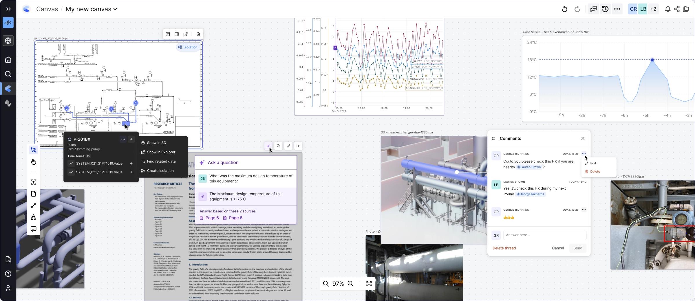
A root-cause analysis in Canvas, step by step:
- Frame it. New canvas "BFP-1A trip 12 Sep". Add a text box with the event description.
- Drop the evidence. Search
BFP-1A→ drag the asset; from its panel drag the P&ID, the last work order, the datasheet. Add the discharge pressure and motor current time series → they render as charts on the canvas; align their time ranges to the trip. - Add the physical view. "Show in 3D" → a 3D card focused on the pump. Add the site photo from the last inspection.
- Cause map. Use the cause-map template (sticky notes with arrows): trip ← high bearing temp ← lube-oil flow low ← filter ΔP high ← filter change overdue (work order postponed).
- Ask Copilot. "Which documents mention the bearing lubrication interval?" — it answers with page citations from the datasheet on the canvas.
- Collaborate. Comment with @mentions; the maintenance planner replies inline; export a summary.
If the P&ID is not parsed, dragging it gives a dead picture. If the time series are not linked to the asset, they do not appear in its panel. If documents are not categorised and linked, Copilot has nothing to cite. Canvas is where the quality of your contextualization becomes visible to everyone — which is why it is a good demo and a good audit.
6.3 InField
InField is the tablet app for operators. Setting it up is a data-engineering job:
| Setup step | What it needs from you |
|---|---|
| Location | Which asset subtree is "this plant / this unit"; the 3D model and 360° images if available; which data sets the app may read. |
| Checklists & templates | A template is a list of tasks tied to assets: "read local pressure gauge at BFP-1A", "check seal leakage", each with an expected reading type (number / OK-NOK / text) and limits. |
| Rounds | Schedule templates as daily/shift rounds; assign to a team. |
| Write-back | Numeric readings become time series datapoints (manual-entry series), NOK checks become events/observations with photos — all linked to the asset, so they show up in Charts and Canvas next to the sensor data. |
The payoff is the "office ↔ field" loop: an engineer sees a rising bearing temperature in Charts, creates an observation task for tonight's round, the operator sees it on the tablet at the pump (with the P&ID and the 3D position), logs the local reading and a photo, and the engineer sees it in the morning — on the same asset.
6.4 Maintain
Maintain is for turnaround and campaign planning: it pulls work orders from SAP/Maximo (through the same extractors), lets planners group them into scopes, simulates duration, crew and cost, checks against the asset hierarchy and 3D for clashes, and pushes the agreed scope back. Prerequisites: a clean work-order extraction (Module 1) mapped to CogniteActivity with functional locations resolved to assets (Module 2).
6.5 Search & 3D
- Search ranks across all resource types; filters by type, data set, time range, metadata; supports saved searches. Aliases in the CDM make
PT-1019find21-PT-1019. - 3D viewer streams the processed model; "Show in 3D" from any asset; clicking an object opens its data; measurements and slicing; point clouds and 360° images side by side.
- A Charts workspace: pump differential head calculation, unit conversion to kPa, work orders overlaid, an alert with a 10-minute minimum duration and you as subscriber.
- A Canvas RCA for one real or invented trip: P&ID, two trends, a document, a photo, a cause map, one Copilot question with a citation, one comment.
- An InField checklist template (dev project with InField enabled): 5 tasks on 3 assets with limits; run it once yourself on a phone/tablet; find the reading in Charts.
Sandbox: 1 and 2 work fully in publicdata.
Consumption: Power BI, Grafana & OData
⏱ 1.5 h- The four consumption paths and which fits which audience
- Connecting Power BI (OData and the REST connector) without exporting CSVs
- Building a per-asset Grafana dashboard with the Cognite data source
- Where Spark / Databricks / Fabric fit
7.1 Power BI
Two connectors exist. The older OData connector ("Cognite Data Fusion (OData)" in Power BI) exposes tables — Assets, Timeseries, Events, Files, Datapoints aggregates, data-model views — at https://{cluster}.cognitedata.com/odata/{version}/projects/{project}; Cognite now marks it deprecated: keep it only for existing reports. All new reports should use the "Cognite Data Fusion (REST API)" connector, which issues GET/POST and GraphQL queries directly, supports every identity provider CDF supports, performs better and reaches all CDF features.
- Get Data → Cognite Data Fusion → enter project and cluster → sign in.
- Pick Datapoints aggregates, not raw datapoints, and filter in the query step (asset subtree, time range, granularity) so the filter is pushed to CDF instead of downloading everything.
- Join to Assets / data-model views by external ID for hierarchy slicers.
- Schedule refresh in the Power BI service with a service-principal login; keep refresh windows aligned with the nightly workflow.
Power BI is not a time-series database. Pull hourly or daily aggregates for the report period and let CDF do the aggregation. If a report needs sub-minute data, it belongs in Charts or Grafana, not Power BI.
7.2 Grafana
Install the Cognite Data Source plugin from the Grafana catalog, configure project + cluster + OAuth2 client credentials (a service principal with read capabilities). Query editors exist for time series (by external ID, by asset subtree, with aggregates), events (as annotations), and data-model GraphQL. The trick for scale: a dashboard variable that lists pumps from a query, so one dashboard serves every pump — combined with Grafana alerting, this is a cheap ops console.
7.3 Spark, Databricks, Fabric
For bulk analytics and data science, CDF offers a Spark data source (read/write CDF resources as DataFrames) and the Microsoft Fabric connector (two-way, OneLake Delta tables ↔ CDF, no copies in RAW). Pattern: model and contextualise in CDF; train models in Databricks/Fabric on CDF data; write predictions back as time series so Charts and Canvas can show them next to the sensors.
- Power BI: daily average discharge pressure and running hours per pump in Unit 2 (or per compressor stage in the sandbox) for the last 90 days, with a hierarchy slicer. Aggregates only; refresh scheduled.
- Grafana: a pump dashboard with a pump drop-down variable, three panels (pressure, current, bearing temperature) and work orders as annotations; one alert rule.
Access management, governance & Level 2 checkpoint
⏱ 2 h- The identity → group → capability → scope chain, precisely
- How to design roles for a plant and implement them as groups
- Space-based access for data models
- Governance habits that keep a project usable after year one
8.1 The chain
The common ACLs: assetsAcl, timeSeriesAcl, eventsAcl, filesAcl, rawAcl, transformationsAcl, extractionPipelinesAcl, functionsAcl, workflowOrchestrationAcl, dataModelsAcl (schema), dataModelInstancesAcl (data), datasetsAcl, groupsAcl, projectsAcl. Actions are per ACL (READ, WRITE, LIST, OWNER…). Scopes: all, datasetScope, spaceIdScope, tableScope (RAW), idScope, assetRootIdScope.
// A CDF group as the API sees it (the UI builds this form; the Toolkit stores it as YAML in Level 3)
{
  "name": "unit2-engineers",
  "sourceId": "3f9c1c2e-…",                                  // Entra ID group object id
  "capabilities": [
    { "timeSeriesAcl":         { "actions": ["READ"],          "scope": { "datasetScope": { "ids": [4501] } } } },
    { "assetsAcl":             { "actions": ["READ"],          "scope": { "datasetScope": { "ids": [4501, 4502] } } } },
    { "filesAcl":              { "actions": ["READ"],          "scope": { "datasetScope": { "ids": [4502] } } } },
    { "eventsAcl":             { "actions": ["READ"],          "scope": { "datasetScope": { "ids": [4503] } } } },
    { "dataModelsAcl":         { "actions": ["READ"],          "scope": { "spaceIdScope": { "spaceIds": ["hnm_power", "cdf_cdm"] } } } },
    { "dataModelInstancesAcl": { "actions": ["READ", "WRITE"], "scope": { "spaceIdScope": { "spaceIds": ["hnm_power_data"] } } } },
    { "projectsAcl":           { "actions": ["LIST"],          "scope": { "all": {} } } }
  ]
}- Scope
allfor convenience. It never gets removed. Scope by data set / space from day one. - Personal accounts for extractors. The person leaves; the pipeline dies. Service principals, one per integration.
- Resources without a data set. They cannot be scoped, so they end up visible to everyone or nobody.
8.2 Designing roles for a plant
| Role (CDF group) | Who | Capabilities (summary) | Scope |
|---|---|---|---|
viewers | Management, most staff | READ on assets, time series, events, files; READ data-model instances | Per-unit data sets / spaces they may see |
unit2-engineers | Process, C&I, reliability | viewers + WRITE instances (Canvas, Charts calcs, annotations approval), events WRITE (observations) | Unit 2 data sets + hnm_power_data |
field-operators | InField users | READ + events/time series WRITE for manual readings | Their unit; the manual-entry data set |
data-engineers | Integration team | RAW, transformations, extraction pipelines, functions, workflows, data models WRITE | All project data sets; schema + data spaces |
extractor-pi, extractor-cmms | Service principals | time series/datapoints WRITE, RAW WRITE on their tables, extraction-pipeline runs WRITE | Exactly their data set / RAW tables — nothing else |
admins | 2–3 people | groups, projects, datasets, everything | all — and audited |
8.3 Data-model access
Two ACLs, two questions: dataModelsAcl — may you read/change the schema (spaces, containers, views, models)? dataModelInstancesAcl — may you read/write the data (nodes, edges)? Both are scoped by space. This is why Module 3 separated hnm_power (schema) from hnm_power_data (data): engineers get WRITE on the data space and READ on the schema; only data engineers change the schema. Remember to include cdf_cdm in READ scopes or CDM-based views will not resolve.
8.4 Governance habits
- Naming conventions written down: data sets
ds_<source>_<unit>, external IDs<source-prefix>:<id>or the plant tag, spaces<org>_<domain>[_data], groups<unit>-<role>. - Data-set descriptions filled in (owner, source system, refresh, contact) — the data catalog is only as good as these.
- Quality checks in transformations (reject rows with null tags into a quarantine RAW table) and a weekly coverage number: % time series linked to an asset, % drawings parsed.
- Change log for the data model: version bumps, what changed, who consumes each view.
- Audit: review admins quarterly; review
all-scoped capabilities monthly (there should be none outside admins).
- Write the role table above for your plant (3 units, the 6 roles). One page.
- In the dev project, create the groups with data-set and space scopes (Admin → Access management → Groups; link to IdP group IDs or, for testing, to a test group).
- Create a service principal for "extractor-cmms" with WRITE only on RAW db
cmmsand theds_cmms_equipmentdata set. - Verify with a test user in
viewersscoped to Unit 2: Search finds Unit 2 assets and not Unit 1; Charts cannot open a Unit 1 series; the data-model view lists onlyhnm_power_datainstances. - Run
client.iam.token.inspect()as that user and read back the effective capabilities.
8.5 Level 2 checkpoint quiz
1. Which extractor kind needs no software on premises?
2. What does is_new('key', lastUpdatedTime) do in a transformation?
3. Why must every transformed row have a stable externalId?
4. A workflow task that must not stop the whole run when it fails should set…
5. The required signature of a Cognite Function is…
6. Which object physically stores property values in data modeling?
7. Why should Pump implement CogniteEquipment?
8. Entity matching returned a 0.62 score. Best practice is…
9. For a Power BI report over 90 days you should pull…
10. Access to data-model instances is scoped by…
★ Level 2 capstone — the Unit 2 feedwater mini-solution
If you did every deliverable, you already have it. Tick what exists in your dev project; each line maps to one module:
- RAW table
cmms.equipment_masterfed by an extractor (or CSV stand-in), registered as extraction pipelineep_cmms_equipmentwith failure notifications (M1) - Transformation
tr_assets(idempotent), Functionfn_running_hours, Workflowwf_nightly_unit2(M2) - Data model
PowerPlant v1with Unit / Pump / Sensor implementing CDM types; instances for U2, BFP-1A/1B, sensors; one edge (M3) - Time series linked to pumps by entity matching; one P&ID parsed and ≥10 annotations approved (M4)
- A notebook that plots 30 days of three sensors with work orders shaded (M5)
- Charts workspace with calculation + alert; Canvas RCA; InField checklist (M6)
- Power BI report and Grafana dashboard on aggregates (M7)
- Six groups with data-set/space scopes; a scoped service principal; verified with a test user (M8)
…you could rebuild all eight lines above in a fresh project in one working day — but you would rather not click through it twice. That reluctance is the right instinct: Level 3 starts by putting every one of these objects into Git with the Cognite Toolkit and deploying them with one command.
Certificates & badges for this level
Glossary additions for Level 2
@view, @container, @import, @relation, implements.updated_at) an extractor uses to fetch only changed rows.